
Predictive Modeling for Perishable Inventories
Enhancing Supply Chain Efficiency
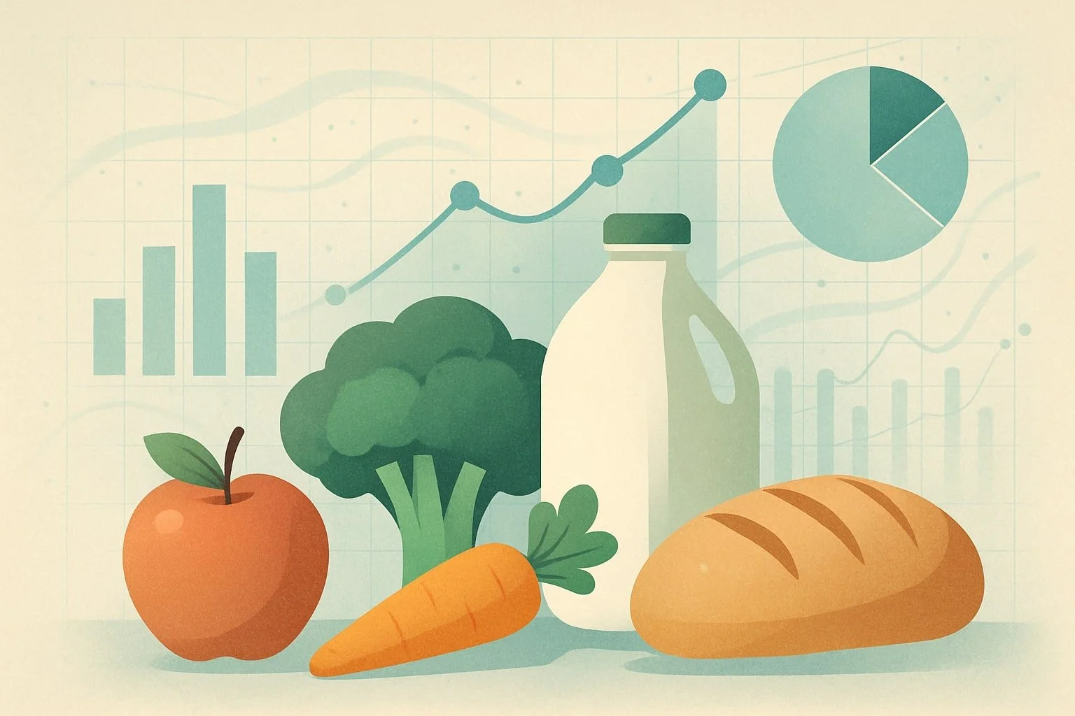
Managing perishable inventory poses a unique challenge for businesses, requiring precise coordination to balance supply with fluctuating consumer demand. Predictive modeling helps organizations anticipate demand patterns for perishable goods, reducing waste and ensuring availability of essential products like food and pharmaceuticals. Data-driven techniques, such as demand forecasting and inventory level analysis, play a crucial role in this process by enabling faster, smarter restocking decisions.
Recent advancements in predictive analytics allow companies to account for consumer preferences, inventory shelf-life, and changing market trends. This targeted approach ensures that inventory levels remain optimized, mitigating the risks associated with spoilage and stockouts.
For businesses handling perishable products, adopting predictive modeling strategies can result in cost savings, improved customer satisfaction, and streamlined operations. Leveraging accurate demand predictions is becoming an essential practice in maintaining an efficient and competitive supply chain.
Fundamentals of Perishable Inventories
Effective management of perishable inventory depends on understanding the nature of products with limited shelf-life, their distinction from non-perishable goods, and the operational features unique to systems handling obsolescence and spoilage. Clear definitions and practical considerations are critical to minimize losses and ensure consistent availability.
Defining Perishable Products
Perishable products are items that have a finite shelf-life and gradually lose value until they become unsellable or unusable. Examples include fresh food, pharmaceuticals, flowers, and some chemicals.
These goods often require special storage conditions such as refrigeration, humidity control, or rapid distribution. Failure to meet these conditions results in reduced quality or total waste.
Obsolescence is also a factor with perishable inventory, as products may become outdated before their physical expiration due to changing consumer preferences or regulations.
Perishable vs. Non-Perishable Inventory
There are several key differences between perishable and non-perishable inventory. Perishable goods degrade over time and present challenges like spoilage, expiration, and variable demand. Non-perishable inventory, such as canned foods or electronics, can be stored for extended periods without significant loss of value.
Feature Perishable Inventory Non-Perishable Inventory Shelf-life Short (hours to months) Long (years) Value Loss Rapid, time-dependent Slow, minimal Storage Requirements Often specialized Standard or minimal Obsolescence Risk High Low to moderate
Inventory systems for perishables must be designed to track aging stock and monitor environmental conditions, while non-perishables focus more on quantity and space management.
Characteristics of Perishable Inventory Systems
Perishable inventory systems include controls for tracking item age, forecasting demand fluctuations, and managing restocking cycles to minimize waste. These systems often incorporate:
First-In, First-Out (FIFO) policies to reduce expiration.
Continuous monitoring of temperature, humidity, and other storage parameters.
Dynamic pricing or markdown strategies to encourage faster turnover as items approach end-of-life.
Limited shelf-life and the possibility of obsolescence require regular assessment. Integration of predictive modeling and real-time data analysis can improve decision-making and lower financial risk by aligning supply with anticipated demand. Inventory rotation and disposal policies are essential for compliance and food safety standards.
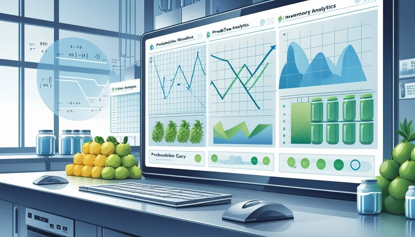
Role of Predictive Modeling in Inventory Management
Predictive modeling enables organizations to accurately forecast demand and manage inventory levels with increased efficiency. This approach directly addresses common challenges faced when handling perishable goods, such as product spoilage, overstock, and understock situations.
Purpose and Benefits of Predictive Models
Predictive models use historical sales data, market trends, seasonal patterns, and real-time information to anticipate future demand. For perishable inventories, this precision is crucial to minimize spoilage and maximize product availability. They also help balance inventory holding costs with customer service levels.
Key benefits include:
Improved demand forecasting accuracy
Reduced waste due to better alignment of stock with actual demand
Optimized replenishment cycles
Cost savings from minimizing excess inventory
By leveraging predictive analytics, businesses can identify slow-moving items early, adjust pricing, and allocate resources effectively. This increases both operational efficiency and profitability, particularly for products with limited shelf life.
Integration with Inventory Control
Predictive modeling is integrated into inventory control systems through automated order generation and real-time inventory tracking. Modern systems often connect with IoT devices, enabling continuous monitoring of product conditions such as temperature for perishable goods.
Integration can include:
Linking predictive models with warehouse management systems
Using early warning alerts to prevent out-of-stock or overstock scenarios
Real-time adjustment of inventory parameters based on current forecasts
Through simulation and continuous feedback, inventory policies adapt quickly to market changes and unexpected demand shifts. This dynamic approach helps ensure that inventory levels are maintained at optimal points, improving both service levels and cost control for perishable inventories.
Key Parameters in Perishable Inventory Models

Accurately predicting inventory needs for perishable goods depends on understanding specific parameters. These parameters affect stock levels, costs, and potential waste, directly influencing operational performance and profitability.
Demand Rate and Demand Function
The demand rate defines how quickly inventory is depleted due to sales or usage. In predictive modeling, demand rates may be stationary (fixed over time) or non-stationary (fluctuating due to trends or seasonality). Identifying the correct demand distribution—whether constant, variable, or exhibiting seasonal patterns—is essential.
Demand functions describe the relationship between inventory level and demand. Forms include additive (demand increases or decreases by a fixed amount) and multiplicative (demand scales based on inventory or price). Models may also account for demand that is sensitive to in-stock quantity or price, especially for items where consumer purchase behavior is affected by stock visibility or product freshness.
Choosing the right demand function and estimating parameters accurately reduce both excess inventory and shortages. This also supports dynamic pricing and real-time inventory adjustments.
Deterioration and Shelf-Life
Deterioration refers to the loss of product usability over time, which is a defining factor in perishable inventory modeling. Shelf-life is the maximum period before an item becomes unsellable or unsafe. Each product may have a unique deterioration rate—some items spoil rapidly while others last longer.
Modeling deterioration typically involves exponential or linear functions, depending on how quickly quality declines. Parameters such as expiration date, storage conditions, and rate of decay must be calibrated for accuracy. If not properly managed, expired stock leads to waste and increased costs.
Inventory policies often require frequent reviews and rotation strategies to minimize expired items. Accurate prediction of shelf-life and deterioration enables efficient stock replenishment and reduces write-offs.
Holding Cost and Time-Varying Costs
Holding cost includes expenses from storing inventory, such as refrigeration, space, insurance, and loss from spoilage. For perishable goods, these costs rise as products approach expiration due to the risk of unsold items and increased chance of spoilage.
Incorporating time-varying costs is crucial. For example, costs may spike during peak seasons or as products near the end of their shelf-life. Some models apply stepped or continuously increasing holding costs to capture this effect.
A breakdown of holding cost components often includes:
Component Example Storage Warehouse, refrigeration Obsolescence Expired product Insurance Theft, damage Capital Tied-up cash
Understanding these costs guides optimal order timing, lot sizing, and markdown strategies, resulting in less waste and improved cost control.
Mathematical Formulation of Predictive Models
Mathematical models for perishable inventory management are used to represent and optimize stock levels, taking into account factors like demand uncertainty and product expiration. The formulation clearly defines variables, constraints, and objective functions to support prediction and decision-making.
Formulating Inventory Control Models
A mathematical model for perishable inventory control typically incorporates demand forecasts, lead times, and perishability constraints. These models use difference equations or stochastic processes to represent daily or period-based inventory changes.
The objective function is often designed to minimize total costs, including ordering, holding, and disposal costs for expired items. Constraints are set to reflect perishability, ensuring that items are used before their expiration.
A standard model may include:
Inventory balance equations
Demand satisfaction requirements
Product age tracking
Mathematical formulations often rely on linear or nonlinear programming methods. In many cases, the use of predictive modeling techniques—such as regression or machine learning—helps refine demand forecasts within the optimization process.
Decision Variables and Constraints
Key decision variables in these models include order quantities at each period, inventory levels by age, and the amount of spoiled or unsold inventory. These variables are selected to ensure effective responses to predicted demand and spoilage.
Common constraints include:
Storage limits: Maximum or minimum inventory allowed, often by product age
Non-negativity: Inventory and orders cannot be negative
Supply and perishability: Items cannot be sold after expiry dates
Typical formulations use the following notation:
Variable Description $x_t^a$ Inventory at time $t$, age $a$ $q_t$ Order quantity at time $t$ $s_t$ Spoiled/expired items at time $t$
These constraints and variables ensure that the mathematical model accurately reflects the realities of perishable inventory systems.
Optimization Techniques for Perishable Inventories
Managing perishable inventories requires balancing order quantities against product lifespans and variable demand. Accurate methods reduce waste and costs, while ensuring product availability and efficiency.
Economic Order Quantity (EOQ) Models
EOQ models offer a formulaic approach to determining the optimal order quantity for perishable products. These models account for factors such as demand rate, lead time, unit cost, and shelf life. Unlike traditional EOQ, perishable EOQ models adjust calculations to incorporate spoilage and time-sensitive demand.
A common approach is the fixed-lifetime model, where products have a set shelf life. The model recommends smaller, more frequent orders than non-perishable EOQ, reducing the risk of items expiring before sale. The table below outlines key differences between classic and perishable EOQ:
Feature Classic EOQ Perishable EOQ Product Lifetime Unlimited Limited (Expires) Order Frequency Lower Higher Spoilage Factor Not included Explicitly included
EOQ-based models serve as a foundation for more advanced optimization methods when handling variable demand and complex supply chains.
Optimal Solution Methods
Optimal solution methods involve analytical and algorithmic techniques that further refine inventory decisions under perishable constraints. Approaches like dynamic programming, Lagrangian relaxation, and scenario-based optimization allow for the incorporation of stochastic demand and uncertain product lifespans.
For example, scenario-based optimization simulates demand variations to identify ordering strategies that minimize total cost and food waste. Lagrangian relaxation can accelerate computations, providing near-optimal order-up-to levels even in large-scale problems. Computational studies have shown that these advanced methods can achieve solutions within 1% of the true optimal cost.
Modern methods may also use deep reinforcement learning models to adapt ordering policies in real time, especially within complex and dynamic retail settings. Each technique aims to find the best balance between ordering costs, spoilage, and service levels.
Modeling Demand Patterns for Perishables
Accurate demand modeling for perishable inventories plays a crucial role in optimizing stock levels and reducing waste. Effective models must account for how demand can change over time or respond non-linearly to outside factors.
Time-Dependent and Quadratic Demand
Perishable goods frequently show demand rates that vary with time, especially for products like fresh foods or seasonal items. Classical models often assume steady demand, but in practice, demand for perishables tends to be time-dependent and sometimes follows a trending or cyclical pattern.
A quadratic demand function is used when changes in demand are not linear. For example, demand may rise rapidly at first, then slow, or even decline after reaching a certain level. This can be modeled mathematically as:
D(t) = a + bt + ct²,
where D(t) is demand at time t, a, b, and c are parameters fitted to historical sales data.
This approach helps inventory planners capture periods of growth and decline, allowing more responsive replenishment or markdown decisions. It is especially useful for products with a strong shelf-life effect or those influenced by promotional campaigns.
Role of the Weibull Distribution
The Weibull distribution is widely used in inventory modeling for perishables to represent product lifetimes and analyze demand uncertainty. Its flexibility allows it to model varying rates of spoilage and consumption over time.
In demand forecasting, the Weibull distribution helps estimate the probability of an item selling before it expires. The distribution is defined by:
Shape parameter (k): Indicates aging effects; higher values mean faster spoilage.
Scale parameter (λ): Represents the expected lifetime of a product.
Typical applications include shelf-life estimation and setting reorder points. By understanding the nature of a product's spoilage with Weibull, supply chain managers can balance stock availability with minimization of outdates. This approach supports both inventory cost reduction and service level targets.
Inventory Cost and Waste Management

Effective management of perishable inventories depends on tracking cost elements and reducing product waste. Understanding calculation methods for inventory-related expenses and handling unsold goods is essential for cost-efficient inventory systems.
Calculating Inventory and Holding Costs
Inventory cost for perishables includes costs of ordering, purchasing, holding, and lost sales due to stock-outs or expiry. Holding cost is influenced by storage duration and product shelf life. Perishables typically have higher holding costs as they require special storage or climate control and lose value over time.
To track these costs, companies may use models that factor in age-based inventory valuation. Some adopt linearly or quadratically time-dependent holding costs. For clarity, a simplified breakdown:
Cost Type Typical Components Holding Cost Storage, insurance, spoilage Inventory Cost Ordering, purchasing, obsolescence
Accurate prediction of these costs helps with pricing and replenishment decisions. Integrating age and expiry into cost models leads to better financial outcomes.
Managing Wastage and Salvage Value
Waste occurs when goods cannot be sold before expiry. Managing this involves timely sales, markdowns, and dynamic inventory controls to reduce unsold stock. Retailers may use predictive models to estimate likely wastage based on demand and shelf life.
Salvage value represents the recovery from expired or unsellable items, such as discounted sales or conversion to secondary products. Including salvage value in inventory models helps offset part of the losses due to waste. Effective strategies may include:
Discounting soon-to-expire stock
Partnering for repurposing surplus products
Using predictive demand models to minimize over-ordering
A balanced approach to waste management and salvage can substantially improve profitability for perishable inventory systems.
Dealing with Demand Uncertainty and Shortages
Managing perishable inventories requires careful attention to both uncertain demand and the consequences of stockouts. Inventory planners must balance maintaining stock availability with the risks and costs associated with shortages and unmet customer needs.
Lost Sales and Unfulfilled Demand
Unfulfilled demand due to stockouts leads directly to lost sales, especially in perishable inventory scenarios where products cannot be backordered indefinitely. Customers may leave for competitors or forego purchases entirely if their needs are not met on time.
Lost sales negatively affect both immediate revenue and longer-term customer loyalty. Predictive models often estimate potential unmet demand by analyzing historical sales patterns, taking into account seasonality and sudden demand changes.
Key strategies to mitigate these lost sales include:
Incorporating real-time demand data into forecasts
Monitoring inventory positions closely
Utilizing safety stock for high-variability items
Sensitivity analysis can help identify the impact of various demand uncertainties. This allows planners to set reorder points that minimize the frequency and impact of missed sales.
Shortage Costs and Backordering
Shortage costs in perishable inventory go beyond lost revenue. These costs can include expedited shipping, process disruptions, and wasted resources from inefficient restocking cycles.
Backordering is less common for perishables, since shelf life limits how long customers are willing to wait. However, some products with moderate perishability may see temporary backorders, leading to additional administrative and customer service costs.
Main cost drivers associated with shortages:
Direct lost revenue
Expedited replenishment fees
Customer compensation or discounts
Increased labor for handling out-of-stock events
Accurate demand forecasts, probabilistic modeling, and Monte Carlo simulations can quantify the likelihood and cost of shortages. These tools enable businesses to determine optimal reorder levels and buffer stocks that minimize total expected shortage costs while balancing freshness and service level targets.
Replenishment and Inventory Policies
Replenishment and inventory management for perishable goods requires careful alignment of policies, demand forecasting, and product shelf-life considerations. These elements play a critical role in minimizing waste, maintaining freshness, and ensuring service levels.
Replenishment Strategies
Replenishment strategies for perishable inventories must address limited shelf life and fluctuating demand. Approaches such as periodic review and continuous review systems are commonly used. In periodic review, orders are placed at fixed intervals, while continuous review triggers replenishment when inventory reaches a set threshold.
Simultaneously optimizing production and routing, especially in multi-echelon networks, can reduce lead times and spoilage. Integrating predictive modeling allows for proactive adjustments based on changing demand patterns and product expiration dates. Policies may factor in variability of lead times and prioritize suppliers with reliable delivery and cold chain capabilities.
FIFO and Freshness Condition
The First-In-First-Out (FIFO) policy helps maintain product freshness and prevents unnecessary spoilage. Under FIFO, older stock is sold or used before newer shipments, aligning movement with the product's age. This method is especially important for items with strict expiration dates, such as food or pharmaceuticals.
Maintaining a record of inventory by age group is crucial for effective FIFO implementation. Technology solutions such as barcode systems and inventory management software can automate tracking and reduce manual errors. Monitoring the freshness condition enables smarter markdowns or targeted promotions for aging stock, supporting both loss reduction and customer satisfaction.
Inventory Control Policy Design
Designing inventory control policies for perishables requires a balance between service levels, holding costs, and product losses due to spoilage. Key policy types include base-stock, order-up-to, and age-based methods that use information about each item's remaining shelf life.
In multi-echelon supply chains, integrated policy models consider replenishment lead times and coordination among warehouses and stores. Predictive analytics can be applied to guide order quantities and timing, taking into account demand variability and seasonality. By employing stochastic modeling and scenario analysis, companies can adapt policies to dynamic supply chain environments, optimizing both costs and product availability.
Applications Across Industries

Predictive modeling for perishable inventories has significant practical use, helping organizations minimize losses, reduce waste, and improve the reliability of supply chains. By basing decisions on analytics and real-time data, companies are better able to manage the unique challenges associated with products that have limited shelf lives.
Retail and Food & Beverage
Retailers and food industry businesses use predictive models to manage inventory levels for perishable items such as dairy, produce, and bakery goods. These models analyze transaction patterns, weather data, and promotions to anticipate demand, helping managers avoid both stockouts and excess inventory.
In grocery and convenience stores, algorithms balance shelf life with consumer buying habits, ensuring fresh products are prioritized for quick sale. Dynamic pricing adjustments are sometimes applied automatically to reduce waste as products approach expiration.
As consumer awareness of food waste increases, chains utilize machine learning and artificial intelligence to further refine forecasts. This allows for smarter ordering, more targeted promotions, and better supplier coordination, supporting both profitability and sustainability goals.
Pharmaceuticals and Medicines
Predictive inventory modeling is essential for pharmaceuticals, where medicines often have short shelf lives and strict storage requirements. Hospitals, clinics, and pharmacies use modeling to ensure necessary drugs are available without overstocking, which reduces the risk of expired stock and financial loss.
For vaccines and temperature-sensitive treatments, real-time monitoring combined with demand forecasting secures product integrity and patient safety. Advanced algorithms can integrate factors such as seasonality, historical dispensation rates, and current health trends to fine-tune inventory levels.
Regulatory compliance is another concern addressed by predictive systems, reducing the likelihood of stockouts or violation penalties. Efficient inventory management in this sector supports continuous patient care and operational efficiency.
Supply Chain and Production Management
Efficient management of perishable inventories depends heavily on the integration of predictive modeling within both supply chain operations and production planning. Technologies such as radio frequency identification (RFID) play a key role by improving real-time tracking and visibility across the value chain.
Integration with Supply Chain Management
Accurate demand forecasting and real-time data sharing are vital for handling perishable goods in the supply chain. Predictive models estimate optimal inventory levels and reorder points, minimizing spoilage and shortages. By accounting for product lifespans and dynamic external factors, these models help companies respond proactively to supply and demand fluctuations.
Integrated supply chain management ensures collaboration between producers, distributors, and retailers. Tools like vendor-managed inventory (VMI) policies promote information sharing and synchronize stock levels. This approach not only reduces waste but also enhances product availability and customer satisfaction.
Benefits of supply chain integration for perishables:
Lower inventory costs
Improved product freshness
Streamlined logistics
Production Planning for Perishables
Production planning for perishable goods must account for shelf life, demand variability, and lead times. Predictive analytics enable manufacturers to align production schedules closely with forecasted demand, reducing overproduction and obsolescence.
Batch sizes and production frequencies can be optimized to balance carrying costs against the risk of spoilage. Simulation models assess scenarios such as sudden demand changes or delays, allowing planners to adjust production runs rapidly. Dynamic scheduling supported by data from the supply chain facilitates attentive and flexible planning.
Key steps in production planning include:
Estimating shelf life and decay rates
Incorporating demand forecasts into schedule adjustments
Evaluating trade-offs between cost and freshness
Role of RFID in Inventory Tracking
Radio frequency identification (RFID) technology provides instant visibility into location, status, and age of inventory throughout the supply chain. RFID tags on products and pallets collect data automatically as items move, reducing manual errors and providing more accurate tracking compared to traditional barcodes.
With real-time tracking capabilities, inventory can be rotated using a first-expiry-first-out (FEFO) strategy, minimizing waste linked to expired goods. RFID data also helps in detecting stockouts and pinpointing inefficiencies in distribution or storage. This leads to faster response times when handling perishable inventory and supports traceability requirements for food safety and regulatory compliance.
RFID enables:
Automated inventory updates
Faster recall processes
Enhanced traceability and compliance
Numerical Examples and Sensitivity Analysis
Numerical examples help clarify model behavior by demonstrating how different inputs affect inventory decisions. Sensitivity analysis further explains the influence of changes in key parameters such as demand rates, deterioration rates, and pricing on inventory performance.
Interpreting Numerical Examples
Numerical examples are constructed by specifying typical parameters—such as shelf life, demand function, cost, and price. These parameters are input into the predictive model to simulate real scenarios faced by inventory managers.
Consider a case for a perishable product with a 10-day shelf life, average daily demand of 100 units, holding costs of $0.20 per item per day, and procurement costs of $2 per unit. Setting an initial selling price at $5, the model determines optimal order quantities and replenishment cycles.
Results might be presented in a table:
Parameter Value Shelf Life (days) 10 Average Demand (units) 100/day Price $5/unit Holding Cost $0.20/unit Order Quantity 950 units Cycle Length 9.5 days Expected Profit/Cycle $2,000
These examples provide tangible insights into how model recommendations align with operational constraints and target profitability.
Conducting Sensitivity Analysis
Sensitivity analysis evaluates how small changes in parameters affect output measures like profit, order quantity, and stock-outs. This process identifies which factors have the most significant impact on performance and guides resource allocation.
Typically, analysts will vary individual parameters—such as increasing the deterioration rate by 10% or decreasing the demand rate—and record the outcomes. For example:
Increasing the deterioration rate from 5% to 8% may reduce order quantities and profit.
Reducing the selling price by $0.50 can lead to higher demand but potentially lower profit margins.
A sample summary may look like this:
Parameter Changed Impact on Profit Impact on Order Quantity Deterioration Rate Increased -12% -10% Demand Rate Increased +18% +15% Price Decreased -9% +20%
These findings help decision-makers prioritize factors that require tighter monitoring or further modeling, ensuring inventory strategies remain robust under varying conditions.
Challenges and Future Directions

Effective predictive modeling for perishable inventories faces persistent challenges related to data and accurate estimation. Meanwhile, the adoption of advanced modeling approaches is changing how organizations address perishability, risk, and uncertainty.
Data Availability and Parameter Estimation
Reliable predictions for perishable inventories require high-quality, granular data on sales, spoilage, shelf life, and external factors like weather or promotions. Many organizations struggle with incomplete or inconsistent records, especially smaller retailers or those with limited digital infrastructure.
Parameter estimation remains a key difficulty. Inaccurate shelf life data or poorly defined demand parameters can quickly degrade model performance. Models rely on accurate forecasts of demand volatility and product decay rates, yet these values often fluctuate by location and season.
A table like the following can help illustrate common data challenges:
Challenge Impact on Modeling Incomplete sales data Poor demand forecasts Inaccurate shelf life Misestimated spoilage Sparse historical data Unreliable parameters
Improving real-time data collection, investment in IoT sensors, and regular calibration of model parameters can address these issues.
Trends in Advanced Predictive Models
Recent years have seen an increase in using machine learning and advanced statistical models for perishable inventory problems. Techniques such as ARIMA for time series, gradient boosting, and deep learning can process diverse signals, including market trends, social media, and weather patterns.
Models increasingly factor in uncertainty by integrating stochastic elements and risk measures like conditional value-at-risk (CVaR) to manage unpredictable demand. Age-based and dynamic shelf life modeling are also becoming more common, allowing better optimization for perishability.
Key trends include:
Integration of external data sources (e.g., weather, social media)
Use of hybrid models combining machine learning with traditional forecasting
Adoption of risk-aware approaches for highly variable demand
These trends are driving more responsive, adaptive inventory strategies for perishable goods.
